The following is a simplified presentation of what GeoSpatial Data is and how it represents Geographic Information. The purpose of this articel is to present the principles of geospatial data. For a more conceptual description of how reality is modded using geospatial data read the article “Representing Reality: How Geographic Information Captures Phenomena“
Put simply spatial data combines the where with the what I.e. it represents information describing what is where. We often use the term GeoSoatial rather in spatial data to emphasise that the were refers to a location on earth (Geo from Greek for earth or land). i.e. not on Mars or in J.R.R. Tolkien’s middle earth. It would also be correct to talk about temporal, geospatial data since all geospatial data includes an implicit or explicit reference to then the where was located where. To avoid the somewhat awkward use of “where” and “what” the what is generally named the attribute data and the where is named locational or positional data. In other words, we often talk about three aspects of GeoSpatial data:
- Attribute data
Represents the what or the properties of the geospatial information. - Locational or positional data
Describes the “where” aspect of the geospatial information. - Temporal data
Temporal data, if used, define a period in time that the combination of attribute and locational data relates to.
One of the key points in the article “Representing Reality: How Geographic Information Captures Phenomena” is that there are two fundamentally different categories of geographic information, namely entities and property fields. An entity is, in this context, defined as something, for instance, a building that has a well-defined extent in time and space and where the same attribute data can apply to the entire extent. A property field is, in this context, defined as a property (attribute) that varies continuously as a function of the location, for instance, elevation above sea level.
When representing entity-based geographic information, for instance, describing a building, attribute data could describe the material of the roof of the building. The locational data describes the location/extent of the building, and finally, the temporal data describes the time period when the building existed at a given location with the given roof material. The fact that the data describes buildings is often given implicitly through the name of the data set.
In the case of property field-based geographic information, for instance, describing air temperature, the attribute data would be the temperature, the locational data would be the location whose temperature was as described by the attribute data, and finally, the temporal data should be the data and time of day the attribute data refer to. Here the temporal data is often given through the name of the data set I,e, mean air temperature August 2022.
Storing geospatial data
In the following, I will discuss the two main principles used to store geospatial data, namely as vector data or raster data. It is worth noting that both entity and field bases geospatial data can be stored using either the raster or vector data approach. However, there is a tendency for property field-based geoinformation to use the raster data approach and entity-based representations to use the vector storage approach, but the choice of approach depends on many different factors
Vector data.
The principle vector data is to represent the locational aspect using one of three geometry types: points, lines and polygons. 3D polygons are often named meshes.
Points
In an entity-based representation, points are used to represent entities where the extent is considered to be of less importance, typically because it, at the intended scale of use is too small to be of relevance. This could for instance be lampposts, trees or boreholes.
In a field-based representation, points are used to define locations of known attribute values, i.e locations where the elevation above sea level has been measured.
As geometry points are given as (x,y) or (x,y,z) i.e. in either 2 or 3 dimensions where the z typically is the elevations above sea level.
p1 = Point(0,0)
p2 = Point(0,10)
p3 = Point(10,10)
p4 = Point(10,0)
p5 = Point(5,5)
A common example of (x,y,z) data is elevation data collected using Lidar where a laser beam from an aeroplane or drone is bounced off the surface of the earth. The output of this method is a collection of (x,y,z) points where z is the elevation above sea level and the attributes among other things include the strength of the returned laser beam. The strength of the returned laser beam can be used to determine the type of surface, brick, soil, vegetation, etc. that reflected the laser beam. This process of using Lidar to determine the election is discussed more in the section on Lidar
Lines
In an entity-based representation, lines are used to represent linear features where the extent in terms of width is of less importance at the internet scale of use. Lines are typically used to for streams, power lines, railroads, roads etc. Roads are a bit of a special case in relation to both route planning and related elements such as bicycle paths and pavements. This is covered in the section on working with transport networks.
In a field-based representation, lines are used to represent lines of an equal attribute value, so-called isolines for instance Contour lines in an elevation data set or Isobars in an air pressure data set. The use of lines in field-based representations are not common and are primarily used for presentation purposes, i.e. human-readable maps rather than computer-based storage.
As geometry lines are represented as a series of points implicitly connected by straight lines segments i.e a line represented by the points (0,0) and (10,10) also includes the point (5,5)
line = LineString([p1,p3])
Polygons
In an entity-based representation, polygons are used to represent entities, where not only the location but also the extent of the entity is important. This could for instance be buildings, forests, municipality etc.
In a field-based representation polygons are used to represent areas with a known constant attribute value for instance lakes in an elevation data set. As with lines, polygons are seldom used in field-based representation
As geometry polygons are represented as series of points implicitly connected by state line segments.
poly = Polygon([p1,p2,p3,p4])
Strictly speaking it is not quite correct to talk about polygons, since in geodata “polygons” can contain both holes and disconnected areas as can be seen below, however, I will stick to the naming practice and call them polygons.

Datasets and attributes
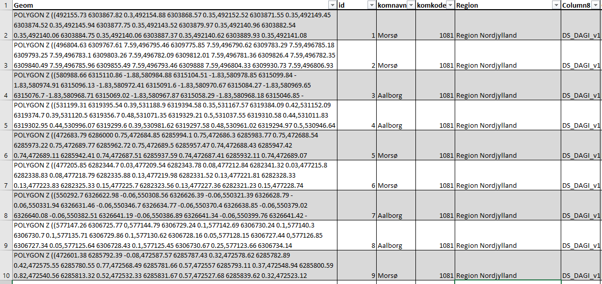
Until now, we have looked at the individual geometries that are used in vector storage, In praxis, these geometries are organized into tables (like spreadsheets) where each attribute is represented by a column and the locational data is represented in an additional column, see Figure 1
Raster data
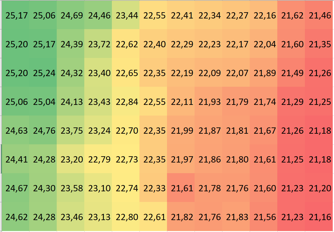
Raster data can be thought of as a grid of evenly spaced vector data points where each has one and only one numerical attribute. It turns out that is this situation it is not nessersary to include the X and Y coordinates of the individual points, only the coordinate of the first point, the distance and direction to the next point and finally how many points there are in a row. Since the points are evenly spaced and in a regular grid this is all you need to calculate the coordinates of all other points. The attribute data are then stored in a table or grid as shown below.
Apart from not needing to explicitly store the X and Y coordinates of the individual points. The fact that each point has one and only one (numerical) attribute means that each point’s attribute data take up the same amount of bytes. While this might sound a bit nerdy, this as actually the largest advantage with raster data. Because the attribute of each point takes up the same amount of bytes it is extremely easy (quick) to look up the attribute values of a point’s neighbouring points. This aspect of raster data makes many types of spatial analysis and especially simulation much quicker using raster data compared to vector data.
When representing entity-based information, entities are either represented by one or more cells containing an identifier of the entity, e.g. a municipality id. or more commonly by a code number representing the type of entity covering the individual cell, e.g. 1 = forest, 2 = building, 3 = lake.
When representing field-based information, each cell contains the value of the attribute being represented at a well-defined location within the cell, typically the centre.
The primary source of raster data are “Image sensors” that produce regular grided point measurements such as multispectral satellite-mounted sensors, Aerial photography or scanned historical topographical maps. Another comment source of raster data is interpolating unregular point data such as Lidar data for creating elevation data (DTM and DSM). For a detailed discussion of surface and elevation data, see the article “Elevation and Surface Modelling“. Finally, you can also convert vector data to raster data in order to support specific types of spatial analysis
Coordinate reference System
Common for both vector and raster data is that it needs a Coordinate Reference System (CRS) that maps the coordinates used in the geospatial data to a location on earth. The CRS is typically defined by giving an ESPG code which is a code value that refers to a well-defined list of CRS definitions. You can read more about how Coordinate Reference Systems in the article “Coordinate Reference Systems”