When working with geospatial data, you often find yourself in a situation where the available data is almost but not quite right. The data might include too many elements, lack an attribute you need or even be too detailed. To overcome this problem, you can use three basic database operations joining, filtering and grouping. In the following, we will look at each of these in turn.
Joining
Joining is used to add additional attributes to your geospatial data, often from a non-geospatial data source, as is the case if you want to visualise statistical data as a map. The typical situation is that your geospatial data contains the geometry of the statistical units, e.g. municipalities or countries, together with an identifier for each unit such as a name or code. Your statistical (non-spatial data) contains the same identifier in addition to attributes representing the statistical values for the unit, i.e. average income. Suppose you think of your data as tables as below. What a join does is that it joins the two tables into one wider table by appending the rows from one table to the end of the rows of the other table where the identifiers (name or code) match.
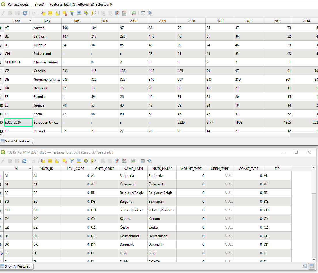
The top table is a Eurostat statistical table of rail accidents by country (NUTS 0) the bottom table is a geospatial dataset of the EU countries (NUTS 0)
These two tables can be joined based on the “id” attribute from the NUTS table and the “CODE” attribute from the rail accidents table, resulting in the table below.
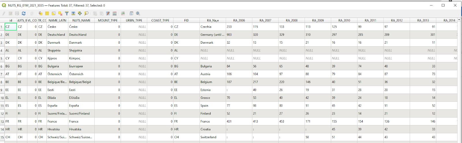
The two tables from figure 8 joined based on the id attribute from the geospatial data table matching the code attribute from the statistical table. The names of all attributes from the statistical table are prefixed with “RA_”
Filtering
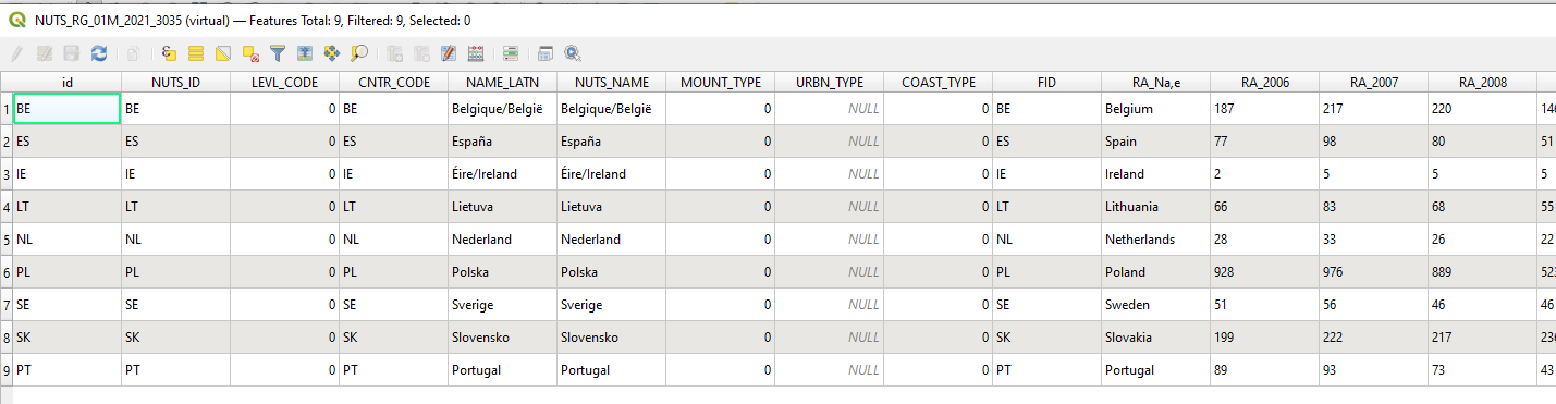
Filtering is the process of removing all rows that do not meet a specific set of criteria. In the case of the rail accidents, we could be interested in looking at which countries had more accidents in 2007 than in 2006. This is achieved by creating a filter that states that we only want the rows where the attribute RA_2007 is larger than RA_2006 (RA_2007 > RA_2006)
Resulting in 9 rows.
Grouping
Grouping is used if you want to aggregate some or all the rows.
In the example of the rail accidents, I have added an attribute named nordic that has the value of 1 for the Nordic countries and 0 for all other countries.
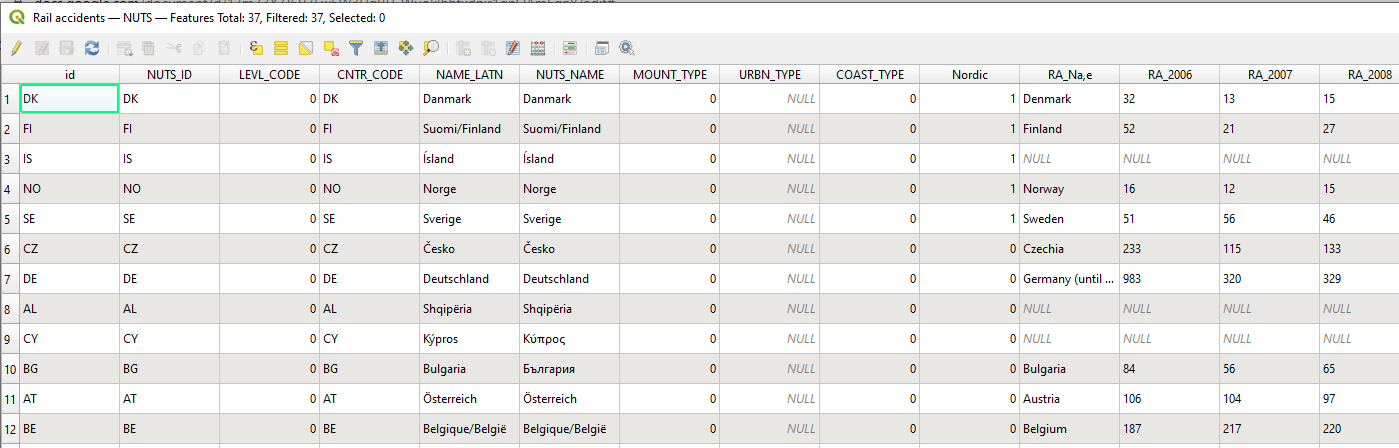
If we now want to know how the sum and average of accidents for the Nordic countries and in the non-nordic countries for the year 2006 we can summerise the attribute RA_2006 on the groups defined by the attribute Nordic
The result would look something like
| Nordic | count | sum | mean |
| 1 | 4 | 151 | 37,75 |
| 0 | 21 | 5136 | 244,57 |
Joining, filtering, and Grouping are all based on the database query language SQL (Structured Query Language), which is the most common way to operate on relational databases. You can find a more detailed description in the posts “Filtering by attribute values”, “Joining attribute data”, and Statistics by Groups